Ozone exposure and health data analysis • bspme

This is a vignette for the bspme package based on ozone exposure data of midwest US, 1987 and simulated health dataset.

First load the package and data:

rm(list=ls())
library(bspme)
library(fields)
data(ozone)
data(health_sim)

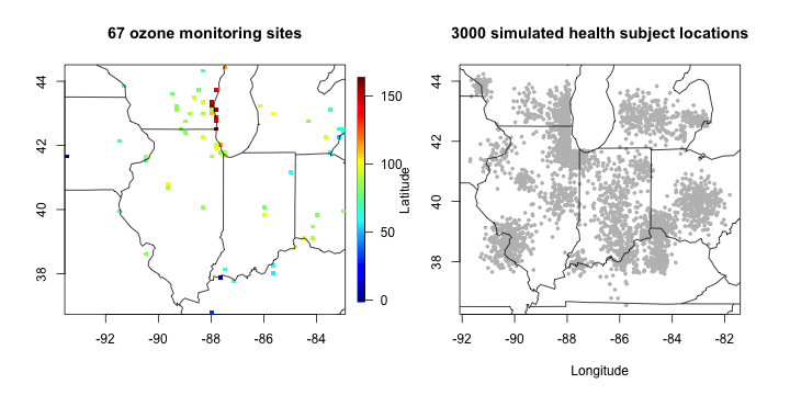
The ozone data are collected daily at 67 monitoring sites in midwest US during 89 days. We focus on ozone exposure on a specific date 06/18/1987 (date id = 16). We also consider simulated health dataset, with \(n=3000\) subject locations and continuous health responses.

ozone16 = ozone[ozone$date_id==16,]
par(mfrow = c(1,2))
quilt.plot(cbind(ozone16$coords_lon, ozone16$coords_lat),
           ozone16$ozone_ppb, main = "67 ozone monitoring sites"); US(add= T)
plot(health_sim$coords_y_lon, health_sim$coords_y_lat, pch = 19, cex = 0.5, col = "grey",
     xlab = "Longitude", ylab = "Latitude", main = "3000 simulated health subject locations"); US(add = T)

plot of chunk ozone_eda

Obtain posterior predictive distribution at health subject locations

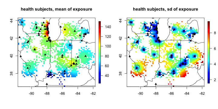
In this example, we will use Gaussian process to obtain a predictive distribution of \((X_1,\dots,X_n)\), the ozone exposure at the health subject locations. The posterior predictive distribution is n-dimensional multivariate normal \(N(\mu_X, Q_X^{-1})\), which will be used as a prior in health model to incorporate measurement error information of ozone exposure. Specifically, we will use the exponential covariance kernel with fixed range 300 (in miles) and standard deviation 15 (in ppb).


# distance calculation
Dxx = rdist.earth(cbind(ozone16$coords_lon, ozone16$coords_lat))
Dyy = rdist.earth(cbind(health_sim$coords_y_lon, health_sim$coords_y_lat))
Dxy = rdist.earth(cbind(ozone16$coords_lon, ozone16$coords_lat),
                  cbind(health_sim$coords_y_lon, health_sim$coords_y_lat))

# kernel matrices
Kxx = Exponential(Dxx, range = 300, phi=15^2)
Kyy = Exponential(Dyy, range = 300, phi=15^2)
Kxy = Exponential(Dxy, range = 300, phi=15^2)

# posterior predictive mean and covariance
X_mean = t(Kxy) %*% solve(Kxx, ozone16$ozone_ppb)
X_cov = Kyy - t(Kxy) %*% solve(Kxx, Kxy)

# visualization of posterior predictive distribution. Black triangle is monitoring station locations.
par(mfrow = c(1,2))
quilt.plot(cbind(health_sim$coords_y_lon, health_sim$coords_y_lat),
           X_mean, main = "health subjects, mean of exposure"); US(add= T)
points(cbind(ozone16$coords_lon, ozone16$coords_lat), pch = 17)

quilt.plot(cbind(health_sim$coords_y_lon, health_sim$coords_y_lat),
           sqrt(diag(X_cov)), main = "health subjects, sd of exposure"); US(add= T)
points(cbind(ozone16$coords_lon, ozone16$coords_lat), pch = 17)

plot of chunk ozone_eda3

The covariance of \((X_1,\dots,X_n)\) contains all spatial dependency information up to a second order, but its inverse \(Q_X\) become a dense matrix. When it comes to fitting the Bayesian linear model with measurement error, the naive implementation with n-dimensional multivariate normal prior \(N(\mu_X, Q_X^{-1})\) takes cubic time complexity of posterior inference for each MCMC iteration, which becomes infeasible to run when \(n\) is large such as tens of thousands.

Run Vecchia approximation to get sparse precision matrix

We propose to use Vecchia approximation to get a new multivariate normal prior of \((X_1,\dots,X_n)\) with sparse precision matrix, which is crucial for scalable implementation of health model with measurement error, but also at the same time it aims to best preserve the spatial dependency information in the original covariance matrix.

#Run the Vecchia approximation to get the sparse precision matrix.

# Vecchia approximation
run_vecchia = vecchia_cov(X_cov, coords = cbind(health_sim$coords_y_lon, health_sim$coords_y_lat),
            n.neighbors = 10)
Q_sparse = run_vecchia$Q
run_vecchia$cputime
#> Time difference of 0.796325 secs

Fit bspme with sparse precision matrix

We can now fit the main function of bspme package with sparse precision matrix.

# fit the model
fit_me = blinreg_me(Y = health_sim$Y,
              X_mean = X_mean,
              X_prec = Q_sparse, # sparse precision matrix
              Z = health_sim$Z,
              nburn = 100,
              nsave = 1000,
              nthin = 1)

fit_me$cputime
#> Time difference of 6.17423 secs

It took less than 10 seconds to (1) run Vecchia approximation and (2) run the MCMC algorithm with total 1100 iterations.

summary(fit_me$posterior)
#> 
#> Iterations = 1:1000
#> Thinning interval = 1 
#> Number of chains = 1 
#> Sample size per chain = 1000 
#> 
#> 1. Empirical mean and standard deviation for each variable,
#>    plus standard error of the mean:
#> 
#>                 Mean       SD  Naive SE Time-series SE
#> (Intercept) 100.0234 0.624015 0.0197331      0.0259492
#> exposure.1   -0.5021 0.007004 0.0002215      0.0003135
#> covariate.1   4.3374 0.337301 0.0106664      0.0126324
#> sigma2_Y     24.7826 0.712924 0.0225446      0.0280662
#> 
#> 2. Quantiles for each variable:
#> 
#>                2.5%     25%      50%      75%    97.5%
#> (Intercept) 98.8360 99.6014 100.0057 100.4462 101.2774
#> exposure.1  -0.5163 -0.5066  -0.5021  -0.4974  -0.4882
#> covariate.1  3.6657  4.1060   4.3402   4.5681   4.9898
#> sigma2_Y    23.3910 24.3080  24.7964  25.2340  26.1523
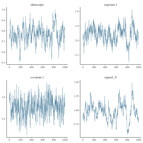
bayesplot::mcmc_trace(fit_me$posterior)

plot of chunk unnamed-chunk-3

Fit bspme without sparse precision matrix

As mentioned before, if precision matrix is dense, the posterior computation becomes infeasible when \(n\) becomes large, such as tens of thousands. See the following example when \(n=3000\).

# fit the model, without vecchia approximation
# I will only run 11 iteration for illustration purpose
Q_dense = solve(X_cov) # inverting 3000 x 3000 matrix, takes some time
# run
fit_me_dense = blinreg_me(Y = health_sim$Y,
                X_mean = X_mean,
                X_prec = Q_dense, # dense precision
                Z = health_sim$Z,
                nburn = 1,
                nsave = 10,
                nthin = 1)

fit_me_dense$cputime
#> Time difference of 58.06338 secs

With even only 11 MCMC iterations, It took about 1 mins to run the MCMC algorithm. If number of health subject locations is tens of thousands, the naive algorithm using dense precision matrix becomes infeasible, and Vecchia approximation becomes necesssary to carry out the inference.